Introduction

The first time I heard the term Random Matrix Theory (RMT) was at the Wednesday physics colloquium given by one of the faculty members at Rutgers. Immediately, I was intrigued by the idea of bringing together two of the most useful concepts in math: statistics and linear algebra. It wasn't obvious to me what we could learn from studying random matrices but the more research I did into the field, the more I realized that their usage was spreading across the different branches of science.

In an effort to learn the basics, I read through multiple sets of lecture notes and articles looking for examples that would build on my background and familiarity with physics. The simplest (and most helpful) example that I found that illustrated the concepts of RMT was the exact result for the 2x2 Gaussian Orthogonal Ensemble (GOE) level repulsion. Before we get into the details and significance of GOE, level repulsion, and other concepts let's take a look at the example.

The 2x2 Example

Random Variables

If you're familiar with statistics, you'll understand the concept of random variables. To summarize, a random variable $X$ is one whose value is sampled from a distribution. The classic examples of discrete random variables are the result of a coin toss or dice roll. Examples of continuous random variables are those that sample from a Gaussian or uniform distribution.

In any case, a normally distributed random variable is often written as $X\sim\mathcal{N}(\mu,\sigma^2)$ meaning that the values of $X$ are sampled from a Gaussian distribution with mean $\mu$ and standard deviation $\sigma$. In other words the probability density function (pdf) of $X$, $f_X(x)$, is given by \begin{equation} f_X(x) = \frac{1}{\sqrt{2\pi\sigma^2}}\exp \left[-\frac{(x-\mu)^2}{2\sigma^2}\right] \end{equation} so that the probability that the value of $X$ lies between $a$ and $b$ is given by \begin{equation} \Pr[a \leq X \leq b] = \int_a^b dx f_X(x). \end{equation}

Random Matrices

With the concept of random variables, we can now introduce a random matrix. A random matrix is simply a matrix whose entries are random variables. The Gaussian Orthogonal Ensemble mentioned before is an ensemble of real symmetric random matrices whose entries are normally distributed random variables. Consider the GOE containing matrices of the form \begin{equation} \begin{bmatrix}X_1 & X_3 \\X_3 & X_2\end{bmatrix} \label{eq:goe} \end{equation} with $X_1\sim\mathcal{N}(0,1)$, $X_2\sim\mathcal{N}(0,1)$, and $X_3\sim\mathcal{N}(0,\frac{1}{2})$. Sampling from this ensemble will give matrices that look like \begin{equation} \begin{bmatrix}0.554030 & -0.471710 \\ -0.471710 & -0.124200\end{bmatrix} \end{equation}

Separation Between Eigenvalues

What can we learn from generating matrices from the ensemble described by Eq. $\eqref{eq:goe}$? The answer is usually in the spectral properties, i.e. the properties of the eigenvalues. One question we might like to answer is: what is the typical spacing between eigenvalues?

To approach this problem we need to diagonalize a random matrix. Although this may seem strange it is actually straight forward. Take Eq. \eqref{eq:goe} and do the usual diagonalization procedure i.e. set \begin{equation} \det \begin{bmatrix}(X_1 - \lambda ) & X_3 \\X_3 & (X_2 -\lambda ) \end{bmatrix} = 0 \end{equation} and solve for $\lambda$. For a 2x2 matrix this can be easily solved to give \begin{equation} \lambda_{\pm} = \frac{X_1 + X_2 \pm \sqrt{(X_1-X_2)^2 + 4 X_3^2}}{2} \label{eq:ev}. \end{equation} The spacing, $s$, is then given by \begin{equation} s = \lambda_+ - \lambda_- = \sqrt{(X_1-X_2)^2 + 4 X_3^2} \label{eq:spa}. \end{equation} Since $s$ is a function of random variables, it itself is a random variable and we can find its pdf, i.e. the probability distribution of the spacing between the eigenvalues. This is given by: \begin{equation} p(s) = \int_{-\infty}^{\infty} dx_1 dx_2 dx_3 \frac{e^{-\frac{1}{2}x_1^2}}{\sqrt{2\pi}}\frac{e^{-\frac{1}{2}x_2^2}}{\sqrt{2\pi}}\frac{e^{-x_3^2}}{\sqrt{\pi}}\delta(s-\sqrt{(x_1-x_2)^2 + 4 x_3^2}) \label{eq:psfull} \end{equation} To proceed it is helpful to introduce new variables $r,\theta,\psi$ defined through \begin{equation} \begin{cases} x_1 - x_2 = r\cos(\theta) \\
2x_3 = r\sin(\theta) \\
x_1 + x_2 = \psi \end{cases} \end{equation} Upon substitution into Eq. $\eqref{eq:psfull}$ we obtain \begin{equation} p(s) = \int_{0}^{\infty} dr ~r\delta(s-r) \int_{0}^{2\pi} d\theta \int_{-\infty}^{\infty} d\psi ~e^{-\frac{1}{2}\left[\left(\frac{r\cos(\theta)+\psi}{2}\right)^2+\left(\frac{-r\cos(\theta)+\psi}{2}\right)^2+\frac{r^2\sin^2(\theta)}{2}\right]} \end{equation} \begin{equation} p(s) = \frac{s}{2}e^{-s^2 /4} \end{equation} We can rescale our result by the mean level spacing, $\langle s \rangle = \sqrt{\pi}$ and the final result is known as Wigner's Surmise: \begin{equation} p(s) = \frac{\pi s}{2}e^{-\frac{1}{4}\pi s^2} \label{eq:wigsur} \end{equation} 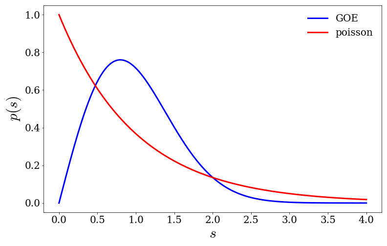From Eq. $\eqref{eq:wigsur}$ we see that the probability that two eigenvalues are either very close together or very far apart vanishes. This behavior is known as level repulsion and is a generic feature of correlated random variables. If we were to look at the probability distribution of the seperation between uncorrelated random variables, we would see something drastically different. In fact, we find that the separation is given by $p(s) = e^{-s}$ and we see that the random variables do not repel but rather attract.

Summary

The idea that we can learn anything by studying random matrices may be quite surprising. At first glance it seems that there is not much to gain by studying a matrix made up of independent random variables. However, by studying the spectral properites of these matrices we find that there are correlations in the spectrum as a result of trading the description of an $N\times N$ matrix of random variables to a description using its $N$ eigenvalues. We have seen level repulsion as one example of many generic features that arise in correlated systems. In physics, the most interesting problems arise when the correlations between the particles are strong and often times random matrix theory finds its way into the description.

The example above is based on the notes by Livan, Novaes, and Vivo